The article contains an introduction to Graph Neural Networks(GNNs) and their applications in Molecular Property Prediction.
Introduction
Deep Learning is suitable for capturing hidden patterns of Euclidean data like images (2D grids) and texts (1D sequences). But what about applications where data is generated from non-Euclidean domains, depicted as graphs with complicated relationships and interdependencies between entities?
That’s where Graph Neural Networks (GNN) come in, which we’ll explore in this article. We’ll start with graph theories and basic definitions, move on to GNN forms and principles, and some applications of GNN and finish with Molecular Property Prediction.
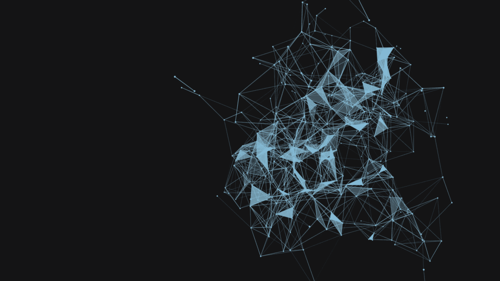
The term GNN is typically referred to a combination of diverse algorithms and not a single architecture. As we will see, a superabundance of diverse architectures has been developed over the years. To give you an early preview, here is a diagram illustrating the most important papers in the field. The diagram has been borrowed from a recent review paper on GNNs by Zhou J. et al.

Different types of Graph Neural Networks. Credits
What is a Graph?
The most fundamental part of GNN is a Graph.
In computer science, a graph is a data structure consisting of two components: nodes (vertices) and edges.
A graph G can be defined as G = (V, E), where V is the set of nodes, and E are the edges between them.
If there are directional dependencies between nodes then edges are directed. If not, edges are undirected.

Directed Graph with nodes and edges. Credits
A graph may be used to describe various objects, including social media networks, city networks, compounds, and molecules. A simple graph might look like this below:

A network graph of the characters in the Game of Thrones. Credits
Graph Neural Networks (GNNs)
Graph Neural Networks(GNNs) are a subclass of Deep Learning approaches that are specially designed to do hypotheses on graph-based data. They are applied to graphs and are adept at performing prediction tasks at the node, edge, and graph levels.

Graph Neural Networks. Credits.
Using graph data any neural network is required to perform tasks using the vertices or nodes of the data. For example, if we are performing any classification job using any of the available GNN then the graph network is needed to classify the vertices or nodes of the graph data. In graph data, nodes should be shown with their labels so that every node can be classified by its labels according to the neural networks.
How GNNs work?
In graph theory, we implement the concept of Node Embedding. which means mapping nodes to a d-dimensional embedding space (low dimensional space rather than the actual dimension of the graph) so that the identical nodes in the graph are implanted close to each other.
The objective here is to map nodes so that similarity in the embedding space resembles similarity in the network.
Let’s define u and v as two nodes in a graph.
xu and xv are two feature vectors.
Next, we’ll define the encoder function Enc(u) and Enc(v), which transform the feature vectors to z_u and z_v.
Note: the similarity function could be Euclidean distance.

So the challenge now is how to come up with the encoder function?
The encoder function should be capable of accomplishing:
Locality (local network neighborhoods)
Aggregate information
Stacking multiple layers (computation)
Locality information can be accomplished by using what we call a computational graph. As shown in the graph below, i is the red node where we see how this node is linked to its neighbors and those neighbors’ neighbors. We’ll see all the possible links, and form a computation graph.
By doing this, we’re grasping the graph skeleton, and also borrowing feature information at the same time.

Neighborhood exploration and information sharing. Credits
Once the locality information holds the computational graph, we start the aggregating process. This is essentially done using neural network architecture.

Consider the above image, On the right is the input graph and a target node A, the graph on the right side shows the computation graph of node A based on its neighborhood. Intuitively, node A acquires all the messages from its neighborhood nodes [B, C, D] and transforms them, and the nodes [B, C, D] in turn transform information from their neighbors. Take a look at the edge directions to comprehend the computational graph. This is a computational graph of depth 2, where original node features of nodes [A, C] are passed to node B, transformed, and then passed again to node A.
The essential intuition is that every node has its own computational graph, and we make use of dynamic recursive programming, and simultaneously calculate node embeddings of all the nodes at each layer of the computational graph and provide them into the next layer of the computational graph.

Every node has a feature vector.
For instance, (X_A) is a feature vector of node A.
The inputs are those feature vectors, and the box will take the two feature vectors (X_A and X_C), aggregate them, and then pass them on to the next layer.
Notice that, for example, the input at node C are the features of node C, but the illustration of node C in layer 1 will be a confidential, latent representation of the node, and in layer 2 it’ll be another latent representation.
So in order to perform forward propagation in this computational graph, we require 3 steps:
1. Initialize the activation units:

2. Every layer in the network:

We can notice that there are two parts to this equation:
The first part is basically averaging all the neighbors of node v.

The second part is the previous layer embedding of node v multiplied with a bias Bk, which is a trainable weight matrix and it’s basically a self-loop activation for node v.

σ: the non-linearity activation that is performed on the two parts.
3. The last equation (at the final layer):

It’s the embedding after K layers of neighborhood aggregation.
Now, to train the model we need to define a loss function on the embeddings.
Training the Model
We can provide the embeddings into any loss function and run stochastic gradient descent to train the weight parameters. For example, for a binary classification job, we can define the loss function as:

Where,
y_v ∈ {0,1} is the node class label.
z_v is the encoder output.
θ is the classification weight.
σ can be the sigmoid function.
σ(z_v^Tθ) represents the predicted probability of node v.
Therefore, the first half of the equation would contribute to the loss function if the label is positive (y_v=1). Otherwise, the second half of the equation would contribute to the loss function.
Training can be unsupervised or supervised:
Unsupervised training: Here we use only the graph layout: similar nodes have similar embeddings. An unsupervised loss function can be a loss based on node nearness in the graph, or random walks.
Supervised training: Train model for a supervised task like node classification, normal or anomalous node.
This is the crux behind the amazing power of Graph Neural Networks. How we aggregate the messages at each level, and how we calculate the message from a node, using all the node neighborhood information are the riffs on our Graph Neural Network.
Why use Graph Neural Networks?
Look around, graphs are all around us, be it the real world or our engineered systems. More often than not, the data we see in machine learning problems is structured or relational, and thus can also be described with a graph. And while fundamental research on GNNs is perhaps decades old, recent advancements in the capabilities of modern GNNs have led to advances in professions as varied as traffic prediction, rumor, and fake news detection, modeling disease spread, physics simulations, and understanding why molecules smell.

Graphs can model the relationships between many different types of data, including web pages (left), social connections (center), or molecules (right). Credits
A graph describes the relations (edges) between a collection of entities (nodes or vertices). We can characterize each node, edge, or the entire graph and store information in each of these pieces of the graph. Additionally, we can ascribe directionality to edges to describe information or traffic flow, for example.
GNNs can be used to answer questions about multiple characteristics of these graphs.
By operating at the graph level, we try to predict the attributes of the whole graph. We can pinpoint the presence of certain “shapes,” like circles in a graph that might describe sub-molecules or possibly close social relationships. GNNs can be used on node-level tasks, to classify the nodes of a graph, and predict partitions and affinity in a graph similar to image classification or segmentation. Finally, we can use GNNs at the edge level to discover connections between entities, perhaps using GNNs to “prune” edges to identify the state of objects in a scene.
Why is it hard to analyze a graph?
Graphs are so complicated that it has begun creating a lot of challenges for current machine learning algorithms.
The reason is that conventional Machine Learning and Deep Learning tools are specialized in simple data types as discussed above. Like images with the same structure and size, we can think of them as fixed-size grid graphs. Text and speech are sequences, so we can think of them as line graphs.
But there are more complex graphs, without a fixed form, with a variable size of unordered nodes, where nodes can have different amounts of neighbors.

It also doesn’t help that existing machine learning algorithms have a core assumption that instances or features are independent of each other. This is false for graph data because each node is related to others by links of various types.
Why do Convolutional Neural Networks (CNNs) fail on graphs?
CNNs can be used to make machines envision things, and perform tasks like image classification, image recognition, or object detection. This is where CNNs are the most prevalent.
The core idea behind CNNs introduces hidden convolution and pooling layers to identify spatially localized features via a set of receptive fields in kernel form.

CNN on an image. Credits
How does convolution operate on images that are regular grids?
We slide the convolutional operator window across a two-dimensional image and compute some function over that sliding window. Then, we pass it through many layers.
Convolution operation on images. Credits
Our objective is to generalize the concept of convolution beyond these simple two-dimensional lattices.
This acuity allows us to reach our objective in that convolution takes a small sub-patch of the image (a little rectangular part of the image), applies a function to it, and produces a new part (a new pixel).
What happens is that the center node of that center pixel aggregates information from its neighbors, as well as from itself, to produce a new value.
It’s very challenging to perform CNN on graphs because of the random size of the graph, and the complicated topology, which means there is no spatial locality.
There’s also an unfixed node arrangement. If we first labeled the nodes A, B, C, D, E, and the second time we labeled them B, D, A, E, and C, then the inputs of the matrix in the network will alter. Graphs are “permutation invariant,” which means changing the order and position of nodes doesn’t make a discrepancy as long as their relations remain the same.
What Functions Can A GNN Perform?
GNNs can be designed to make predictions at the level of nodes, edges, or entire graphs:
Node Classification
Link Prediction
Graph Classification

Node Classification
Predicting the node embedding for each node in a network is what this task entails. Only a portion of the graph is labeled in such circumstances, resulting in a semi-supervised graph. YouTube videos, Facebook friend recommendations, and other applications are examples.
Link Prediction
The primary objective is to determine the relationship between two things in a graph and to forecast if the two entities are connected. Consider a recommender system in which a model is given a collection of user reviews for various items. The objective is to forecast users’ preferences and optimize the recommender system so that it promotes goods that align with the users’ interests.
Graph Classification
It entails sorting the entire graph into a variety of groups. It’s a lot like an image classification problem, however, the goal here is to identify graphs. Examples of Graph Classification include the classification of a chemical structure into one of several categories in chemistry,
Message-passing neural network (MPNN) for molecular property prediction
In this tutorial, we will implement a type of graph neural network (GNN) known as _ message passing neural network_ (MPNN) to predict graph properties. Specifically, we will implement an MPNN to predict a molecular property known as blood-brain barrier permeability (BBBP).
Motivation: as molecules are naturally represented as an undirected graph G = (V, E), where V is a set of vertices (nodes; atoms) and E a set of edges (bonds), GNNs (such as MPNN) are proving to be a useful method for predicting molecular properties.
Until now, more traditional methods, such as random forests, support vector machines, etc., have been commonly used to predict molecular properties. In contrast to GNNs, these traditional approaches often operate on precomputed molecular features such as molecular weight, polarity, charge, number of carbon atoms, etc. Although these molecular features prove to be good predictors for various molecular properties, it is hypothesized that operating on these more "raw", and "low-level", features could prove even better.
Setup
RDKit is a collection of cheminformatics and machine-learning software written in C++ and Python. In this tutorial, RDKit is used to conveniently and efficiently transform SMILES into molecule objects, and then from those obtain sets of atoms and bonds.
SMILES expresses the structure of a given molecule in the form of an ASCII string. The SMILES string is a compact encoding that, for smaller molecules, is relatively human-readable. Encoding molecules as a string both alleviates and facilitates database and/or web searching of a given molecule. RDKit uses algorithms to accurately transform a given SMILES to a molecule object, which can then be used to compute a great number of molecular properties/features.
Notice, that RDKit is commonly installed via Conda. However, thanks to rdkit_platform_wheels, RDKit can now (for the sake of this tutorial) be installed easily via pip, as follows:
!pip install rdkit-pypi
!pip install pandas
!pip install Pillow
!pip install matplotlib
!pip install pydot
!sudo apt-get -qq install graphviz
Import packages
import os

# Temporary suppress tf logs
os.environ["TF_CPP_MIN_LOG_LEVEL"] = "3"

import tensorflow as tf
from tensorflow import keras
from tensorflow.keras import layers
import numpy as np
import pandas as pd
import matplotlib.pyplot as plt
import warnings
from rdkit import Chem
from rdkit import RDLogger
from rdkit.Chem.Draw import IPythonConsole
from rdkit.Chem.Draw import MolsToGridImage

# Temporary suppress warnings and RDKit logs
warnings.filterwarnings("ignore")
RDLogger.DisableLog("rdApp.*")

np.random.seed(42)
tf.random.set_seed(42)
Dataset
Information about the dataset can be found in A Bayesian Approach to in Silico Blood-Brain Barrier Penetration Modeling and MoleculeNet: A Benchmark for Molecular Machine Learning. The dataset will be downloaded from MoleculeNet.org.
About
The dataset contains 2,050 molecules. Each molecule comes with a name, label, and SMILES string.
The blood-brain barrier (BBB) is a membrane separating the blood from the brain's extracellular fluid, hence blocking out most drugs (molecules) from reaching the brain. Because of this, the BBBP has been important to study for the development of new drugs that aim to target the central nervous system. The labels for this data set are binary (1 or 0) and indicate the permeability of the molecules.
csv_path = keras.utils.get_file(
    "BBBP.csv", "https://deepchemdata.s3-us-west-1.amazonaws.com/datasets/BBBP.csv"
)

df = pd.read_csv(csv_path, usecols=[1, 2, 3])
df.iloc[100:107]
Define features
To encode features for atoms and bonds (which we will need later), we'll define two classes: AtomFeaturizer and BondFeaturizer respectively.
To reduce the lines of code, i.e., to keep this tutorial short and concise, only about a handful of (atom and bond) features will be considered: [atom features] symbol (element), number of valence electrons, number of hydrogen bonds, orbital hybridization, [bond features] (covalent) bond type, and conjugation.
class Featurizer:
    def __init__(self, allowable_sets):
        self.dim = 0
        self.features_mapping = {}
        for k, s in allowable_sets.items():
            s = sorted(list(s))
            self.features_mapping[k] = dict(zip(s, range(self.dim, len(s) + self.dim)))
            self.dim += len(s)

    def encode(self, inputs):
        output = np.zeros((self.dim,))
        for name_feature, feature_mapping in self.features_mapping.items():
            feature = getattr(self, name_feature)(inputs)
            if feature not in feature_mapping:
                continue
            output[feature_mapping[feature]] = 1.0
        return output


class AtomFeaturizer(Featurizer):
    def __init__(self, allowable_sets):
        super().__init__(allowable_sets)

    def symbol(self, atom):
        return atom.GetSymbol()

    def n_valence(self, atom):
        return atom.GetTotalValence()

    def n_hydrogens(self, atom):
        return atom.GetTotalNumHs()

    def hybridization(self, atom):
        return atom.GetHybridization().name.lower()


class BondFeaturizer(Featurizer):
    def __init__(self, allowable_sets):
        super().__init__(allowable_sets)
        self.dim += 1

    def encode(self, bond):
        output = np.zeros((self.dim,))
        if bond is None:
            output[-1] = 1.0
            return output
        output = super().encode(bond)
        return output

    def bond_type(self, bond):
        return bond.GetBondType().name.lower()

    def conjugated(self, bond):
        return bond.GetIsConjugated()


atom_featurizer = AtomFeaturizer(
    allowable_sets={
        "symbol": {"B", "Br", "C", "Ca", "Cl", "F", "H", "I", "N", "Na", "O", "P", "S"},
        "n_valence": {0, 1, 2, 3, 4, 5, 6},
        "n_hydrogens": {0, 1, 2, 3, 4},
        "hybridization": {"s", "sp", "sp2", "sp3"},
    }
)

bond_featurizer = BondFeaturizer(
    allowable_sets={
        "bond_type": {"single", "double", "triple", "aromatic"},
        "conjugated": {True, False},
    }
)
Generate graphs
Before we can generate complete graphs from SMILES, we need to implement the following functions:
molecule_from_smiles, which takes as input a SMILES and returns a molecule object. This is all handled by RDKit.
graph_from_molecule, which takes as input a molecule object and returns a graph, represented as a three-tuple (atom_features, bond_features, pair_indices). For this, we will make use of the classes defined previously.
Finally, we can now implement the function graphs_from_smiles, which applies a function (1) and subsequently (2) on all SMILES of the training, validation, and test datasets.
Notice: although scaffold splitting is recommended for this data set (see here), for simplicity, simple random splittings were performed.
def molecule_from_smiles(smiles):
    # MolFromSmiles(m, sanitize=True) should be equivalent to
    # MolFromSmiles(m, sanitize=False) -> SanitizeMol(m) -> AssignStereochemistry(m, ...)
    molecule = Chem.MolFromSmiles(smiles, sanitize=False)

    # If sanitization is unsuccessful, catch the error, and try again without
    # the sanitization step that caused the error
    flag = Chem.SanitizeMol(molecule, catchErrors=True)
    if flag != Chem.SanitizeFlags.SANITIZE_NONE:
        Chem.SanitizeMol(molecule, sanitizeOps=Chem.SanitizeFlags.SANITIZE_ALL ^ flag)

    Chem.AssignStereochemistry(molecule, cleanIt=True, force=True)
    return molecule


def graph_from_molecule(molecule):
    # Initialize graph
    atom_features = []
    bond_features = []
    pair_indices = []

    for atom in molecule.GetAtoms():
        atom_features.append(atom_featurizer.encode(atom))

        # Add self-loops
        pair_indices.append([atom.GetIdx(), atom.GetIdx()])
        bond_features.append(bond_featurizer.encode(None))

        for neighbor in atom.GetNeighbors():
            bond = molecule.GetBondBetweenAtoms(atom.GetIdx(), neighbor.GetIdx())
            pair_indices.append([atom.GetIdx(), neighbor.GetIdx()])
            bond_features.append(bond_featurizer.encode(bond))

    return np.array(atom_features), np.array(bond_features), np.array(pair_indices)


def graphs_from_smiles(smiles_list):
    # Initialize graphs
    atom_features_list = []
    bond_features_list = []
    pair_indices_list = []

    for smiles in smiles_list:
        molecule = molecule_from_smiles(smiles)
        atom_features, bond_features, pair_indices = graph_from_molecule(molecule)

        atom_features_list.append(atom_features)
        bond_features_list.append(bond_features)
        pair_indices_list.append(pair_indices)

    # Convert lists to ragged tensors for tf.data.Dataset later on
    return (
        tf.ragged.constant(atom_features_list, dtype=tf.float32),
        tf.ragged.constant(bond_features_list, dtype=tf.float32),
        tf.ragged.constant(pair_indices_list, dtype=tf.int64),
    )


# Shuffle array of indices ranging from 0 to 2049
permuted_indices = np.random.permutation(np.arange(df.shape[0]))

# Train set: 80 % of data
train_index = permuted_indices[: int(df.shape[0] * 0.8)]
x_train = graphs_from_smiles(df.iloc[train_index].smiles)
y_train = df.iloc[train_index].p_np

# Valid set: 19 % of data
valid_index = permuted_indices[int(df.shape[0] * 0.8) : int(df.shape[0] * 0.99)]
x_valid = graphs_from_smiles(df.iloc[valid_index].smiles)
y_valid = df.iloc[valid_index].p_np

# Test set: 1 % of data
test_index = permuted_indices[int(df.shape[0] * 0.99) :]
x_test = graphs_from_smiles(df.iloc[test_index].smiles)
y_test = df.iloc[test_index].p_np
Test the functions
print(f"Name:\t{df.name[100]}\nSMILES:\t{df.smiles[100]}\nBBBP:\t{df.p_np[100]}")
molecule = molecule_from_smiles(df.iloc[100].smiles)
print("Molecule:")
molecule
graph = graph_from_molecule(molecule)
print("Graph (including self-loops):")
print("\tatom features\t", graph[0].shape)
print("\tbond features\t", graph[1].shape)
print("\tpair indices\t", graph[2].shape)
Create a tf.data.Dataset
In this tutorial, the MPNN implementation will take as input (per iteration) a single graph. Therefore, given a batch of (sub)graphs (molecules), we need to merge them into a single graph (we'll refer to this graph as a global graph). This global graph is a disconnected graph where each subgraph is completely separated from the other subgraphs.
def prepare_batch(x_batch, y_batch):
    """Merges (sub)graphs of batch into a single global (disconnected) graph
    """

    atom_features, bond_features, pair_indices = x_batch

    # Obtain number of atoms and bonds for each graph (molecule)
    num_atoms = atom_features.row_lengths()
    num_bonds = bond_features.row_lengths()

    # Obtain partition indices (molecule_indicator), which will be used to
    # gather (sub)graphs from global graph in model later on
    molecule_indices = tf.range(len(num_atoms))
    molecule_indicator = tf.repeat(molecule_indices, num_atoms)

    # Merge (sub)graphs into a global (disconnected) graph. Adding 'increment' to
    # 'pair_indices' (and merging ragged tensors) actualizes the global graph
    gather_indices = tf.repeat(molecule_indices[:-1], num_bonds[1:])
    increment = tf.cumsum(num_atoms[:-1])
    increment = tf.pad(tf.gather(increment, gather_indices), [(num_bonds[0], 0)])
    pair_indices = pair_indices.merge_dims(outer_axis=0, inner_axis=1).to_tensor()
    pair_indices = pair_indices + increment[:, tf.newaxis]
    atom_features = atom_features.merge_dims(outer_axis=0, inner_axis=1).to_tensor()
    bond_features = bond_features.merge_dims(outer_axis=0, inner_axis=1).to_tensor()

    return (atom_features, bond_features, pair_indices, molecule_indicator), y_batch


def MPNNDataset(X, y, batch_size=32, shuffle=False):
    dataset = tf.data.Dataset.from_tensor_slices((X, (y)))
    if shuffle:
        dataset = dataset.shuffle(1024)
    return dataset.batch(batch_size).map(prepare_batch, -1).prefetch(-1)
Model
The MPNN model can take on various shapes and forms. In this tutorial, we will implement an MPNN based on the original paper Neural Message Passing for Quantum Chemistry and DeepChem's MPNNModel. The MPNN of this tutorial consists of three stages: message passing, readout, and classification.
Message passing
The message passing step itself consists of two parts:
The edge network, which passes messages from 1-hop neighbors w_{i} of v to v, based on the edge features between them (e_{vw_{i}}), resulting in an updated node (state) v'. w_{i} denotes the i:th neighbor of v.
The gated recurrent unit (GRU), takes as input the most recent node state and updates it based on previous node states. In other words, the most recent node state serves as the input to the GRU, while the previous node states are incorporated within the memory state of the GRU. This allows information to travel from one node state (e.g., v) to another (e.g., v'').
Importantly, steps (1) and (2) are repeated for k steps, and where at each step 1...k, the radius (or a number of hops) of aggregated information from v increases by 1.
class EdgeNetwork(layers.Layer):
    def build(self, input_shape):
        self.atom_dim = input_shape[0][-1]
        self.bond_dim = input_shape[1][-1]
        self.kernel = self.add_weight(
            shape=(self.bond_dim, self.atom_dim * self.atom_dim),
            initializer="glorot_uniform",
            name="kernel",
        )
        self.bias = self.add_weight(
            shape=(self.atom_dim * self.atom_dim), initializer="zeros", name="bias",
        )
        self.built = True

    def call(self, inputs):
        atom_features, bond_features, pair_indices = inputs

        # Apply linear transformation to bond features
        bond_features = tf.matmul(bond_features, self.kernel) + self.bias

        # Reshape for neighborhood aggregation later
        bond_features = tf.reshape(bond_features, (-1, self.atom_dim, self.atom_dim))

        # Obtain atom features of neighbors
        atom_features_neighbors = tf.gather(atom_features, pair_indices[:, 1])
        atom_features_neighbors = tf.expand_dims(atom_features_neighbors, axis=-1)

        # Apply neighborhood aggregation
        transformed_features = tf.matmul(bond_features, atom_features_neighbors)
        transformed_features = tf.squeeze(transformed_features, axis=-1)
        aggregated_features = tf.math.unsorted_segment_sum(
            transformed_features,
            pair_indices[:, 0],
            num_segments=tf.shape(atom_features)[0],
        )
        return aggregated_features


class MessagePassing(layers.Layer):
    def __init__(self, units, steps=4, **kwargs):
        super().__init__(**kwargs)
        self.units = units
        self.steps = steps

    def build(self, input_shape):
        self.atom_dim = input_shape[0][-1]
        self.message_step = EdgeNetwork()
        self.pad_length = max(0, self.units - self.atom_dim)
        self.update_step = layers.GRUCell(self.atom_dim + self.pad_length)
        self.built = True

    def call(self, inputs):
        atom_features, bond_features, pair_indices = inputs

        # Pad atom features if number of desired units exceeds atom_features dim.
        # Alternatively, a dense layer could be used here.
        atom_features_updated = tf.pad(atom_features, [(0, 0), (0, self.pad_length)])

        # Perform a number of steps of message passing
        for i in range(self.steps):
            # Aggregate information from neighbors
            atom_features_aggregated = self.message_step(
                [atom_features_updated, bond_features, pair_indices]
            )

            # Update node state via a step of GRU
            atom_features_updated, _ = self.update_step(
                atom_features_aggregated, atom_features_updated
            )
        return atom_features_updated
Readout
When the message passing procedure ends, the k-step-aggregated node states are to be partitioned into subgraphs (corresponding to each molecule in the batch) and subsequently reduced to graph-level embeddings. In the original paper, a set-to-set layer was used for this purpose. In this tutorial, however, a transformer encoder + average pooling will be used. Specifically:
the k-step-aggregated node states will be partitioned into the subgraphs (corresponding to each molecule in the batch);
each subgraph will then be padded to match the subgraph with the greatest number of nodes, followed by a tf.stack(...);
the (stacked padded) tensor, encoding subgraphs (each subgraph containing a set of node states), are masked to make sure the paddings don't interfere with training;
finally, the tensor is passed to the transformer followed by average pooling.
class PartitionPadding(layers.Layer):
    def __init__(self, batch_size, **kwargs):
        super().__init__(**kwargs)
        self.batch_size = batch_size

    def call(self, inputs):

        atom_features, molecule_indicator = inputs

        # Obtain subgraphs
        atom_features_partitioned = tf.dynamic_partition(
            atom_features, molecule_indicator, self.batch_size
        )

        # Pad and stack subgraphs
        num_atoms = [tf.shape(f)[0] for f in atom_features_partitioned]
        max_num_atoms = tf.reduce_max(num_atoms)
        atom_features_stacked = tf.stack(
            [
                tf.pad(f, [(0, max_num_atoms - n), (0, 0)])
                for f, n in zip(atom_features_partitioned, num_atoms)
            ],
            axis=0,
        )

        # Remove empty subgraphs (usually for last batch in dataset)
        gather_indices = tf.where(tf.reduce_sum(atom_features_stacked, (1, 2)) != 0)
        gather_indices = tf.squeeze(gather_indices, axis=-1)
        return tf.gather(atom_features_stacked, gather_indices, axis=0)


class TransformerEncoderReadout(layers.Layer):
    def __init__(
        self, num_heads=8, embed_dim=64, dense_dim=512, batch_size=32, **kwargs
    ):
        super().__init__(**kwargs)

        self.partition_padding = PartitionPadding(batch_size)
        self.attention = layers.MultiHeadAttention(num_heads, embed_dim)
        self.dense_proj = keras.Sequential(
            [layers.Dense(dense_dim, activation="relu"), layers.Dense(embed_dim),]
        )
        self.layernorm_1 = layers.LayerNormalization()
        self.layernorm_2 = layers.LayerNormalization()
        self.average_pooling = layers.GlobalAveragePooling1D()

    def call(self, inputs):
        x = self.partition_padding(inputs)
        padding_mask = tf.reduce_any(tf.not_equal(x, 0.0), axis=-1)
        padding_mask = padding_mask[:, tf.newaxis, tf.newaxis, :]
        attention_output = self.attention(x, x, attention_mask=padding_mask)
        proj_input = self.layernorm_1(x + attention_output)
        proj_output = self.layernorm_2(proj_input + self.dense_proj(proj_input))
        return self.average_pooling(proj_output)
Message Passing Neural Network (MPNN)
It is now time to complete the MPNN model. In addition to the message passing and readout, a two-layer classification network will be implemented to make predictions of BBBP.
def MPNNModel(
    atom_dim,
    bond_dim,
    batch_size=32,
    message_units=64,
    message_steps=4,
    num_attention_heads=8,
    dense_units=512,
):

    atom_features = layers.Input((atom_dim), dtype="float32", name="atom_features")
    bond_features = layers.Input((bond_dim), dtype="float32", name="bond_features")
    pair_indices = layers.Input((2), dtype="int32", name="pair_indices")
    molecule_indicator = layers.Input((), dtype="int32", name="molecule_indicator")

    x = MessagePassing(message_units, message_steps)(
        [atom_features, bond_features, pair_indices]
    )

    x = TransformerEncoderReadout(
        num_attention_heads, message_units, dense_units, batch_size
    )([x, molecule_indicator])

    x = layers.Dense(dense_units, activation="relu")(x)
    x = layers.Dense(1, activation="sigmoid")(x)

    model = keras.Model(
        inputs=[atom_features, bond_features, pair_indices, molecule_indicator],
        outputs=[x],
    )
    return model


mpnn = MPNNModel(
    atom_dim=x_train[0][0][0].shape[0], bond_dim=x_train[1][0][0].shape[0],
)

mpnn.compile(
    loss=keras.losses.BinaryCrossentropy(),
    optimizer=keras.optimizers.Adam(learning_rate=5e-4),
    metrics=[keras.metrics.AUC(name="AUC")],
)

keras.utils.plot_model(mpnn, show_dtype=True, show_shapes=True)
Training
train_dataset = MPNNDataset(x_train, y_train)
valid_dataset = MPNNDataset(x_valid, y_valid)
test_dataset = MPNNDataset(x_test, y_test)

history = mpnn.fit(
    train_dataset,
    validation_data=valid_dataset,
    epochs=40,
    verbose=2,
    class_weight={0: 2.0, 1: 0.5},
)

plt.figure(figsize=(10, 6))
plt.plot(history.history["AUC"], label="train AUC")
plt.plot(history.history["val_AUC"], label="valid AUC")
plt.xlabel("Epochs", fontsize=16)
plt.ylabel("AUC", fontsize=16)
plt.legend(fontsize=16)
Predicting
molecules = [molecule_from_smiles(df.smiles.values[index]) for index in test_index]
y_true = [df.p_np.values[index] for index in test_index]
y_pred = tf.squeeze(mpnn.predict(test_dataset), axis=1)

legends = [f"y_true/y_pred = {y_true[i]}/{y_pred[i]:.2f}" for i in range(len(y_true))]
MolsToGridImage(molecules, molsPerRow=4, legends=legends)
You can download the code from Github.
Conclusion
Graph neural networks are very powerful tools. They have already found powerful applications in domains such as route planning, fraud detection, network optimization, and drug research. Wherever there is a graph of related entities, GNNs can help get the most value from the existing data.
We also demonstrated a message passing neural network (MPNN) to predict blood-brain barrier permeability (BBBP) for a number of different molecules. We first had to construct graphs from SMILES, then build a Keras model that could operate on these graphs, and finally, train the model to make the predictions.
Thank you for reading!